Understanding and building a simple benchmark#

Are you looking for a simple, step-by-step introduction to the Benchopt library? Then look no further! In this tutorial, we are going to learn how to use the Benchopt library to compare various algorithms in order to minimize a given cost. This tutorial complements the write a benchmark webpage with a more practical, hands-on approach.

Let’s say you are interested in benchmarking solvers to minimize the cost function of the ridge regression problem, a variant of linear regression which is a common problem in supervised machine learning. This cost function writes as follows:

\[f(\beta) = \frac{1}{2} {\|y - X\beta\|}^2 + \lambda{\|\beta\|}^2\]

where

\(y\) is a vector with \(m\) elements, typically some observations

\(X\) is a matrix with \(m \times n\) elements, typically the regressors

\(\beta\) is a vector with \(n\) elements that we obtain by regressing \(y\) on \(X\).

\(\|\cdot\|\) is the Euclidean norm.

Let us also suppose that we are working with a specific optimization algorithm that aims at solving the ridge regression problem: the gradient descent (GD) algorithm. GD is a simple algorithm that moves iteratively along the steepest descent direction. Given an estimate \(\beta\), GD iterates the following step:

\[\beta \leftarrow \beta - \eta \nabla f(\beta)\]

where \(\eta\) is the learning rate or stepsize, and controls how much the iterate is moved alongside the descent direction. The vector \(\nabla f(\beta)\) is the gradient of the cost function defined above, evaluated at \(\beta\).

Ridge regression computed with GD is overall a simple procedure, however we should be mindful of the two hyperparameters: the regularization parameter \(\lambda\), and the gradient stepsize \( \eta\). It is very common in machine learning that we are facing a situation where we want to vary these parameters, and compare the behavior of our algorithm in each scenario. Benchopt we can create a benchmark for this problem, here is a screenshot of what we will get at the end of this tutorial.

../_images/screenshot_mytemplate_ridgeloss.png

We can now dive into the framework and see how to leverage it to easily create our benchmark!

Installing Benchopt#

Let’s start by installing the benchopt package. It is a python package, so we are assuming that you are starting this tutorial with a functioning python installation. It is recommended to run all this tutorial in a dedicated environment (such as a virtual environment or a conda environment)

Benchopt can be installed simply using pip by running in a terminal

pip install -U benchopt

Benchopt and its dependencies are going to be installed, just wait until this is done. If you have any issue with the installation, you may have a look at the installation page.

Installing and running a first benchmark#

Benchopt in itself is like a mother package: it supervises and runs smaller libraries, a.k.a. the benchmarks. Therefore, benchmarks are repositories with a predefined structure and some required files (we will go over each of them in the next section) that are processed by benchopt. The benchmark specifies information about:

the problem (typically the loss function to minimize),

the dataset on which the algorithms are tested (values of \(X \) and \( y\))

the solvers (like our GD algorithm).

It is likely that if you are reading this tutorial, you are in fact interested in writing and running a benchmark.

To write a benchmark, it is recommended to start from the template benchmark shared in the Benchopt organisation. To get this template and rename it my_benchmark, you can clone it from its Github repository:

git clone git@github.com:benchopt/template_benchmark my_benchmark

The template benchmark is not designed to model our ridge regression problem, but luckily it is pretty close! The cost which is implemented in the template benchmark is the Ordinary Least Squares (OLS)

\[g(\beta) = \frac{1}{2} \|y - X\beta \|^2\]

and the only implemented solver is GD with \(\nabla g(\beta) = -X^Ty + X^TX\beta \) the gradient of \(g\) at \(\beta \).

We will modify this template to adapt it to the ridge regression problem next, but before that let us run this benchmark. In other words, let us use benchopt to read the contents of the template benchmark and run GD on OLS. The solver will use a predefined set of stepsizes, in our case \( [1, 1.99] \) (the stepsize is scaled by the inverse of the gradient’s Lipschitz constant, you can ignore this detail if you are not familiar with this concept).

To run the template benchmark, simply run the following command in the terminal:

benchopt run my_benchmark

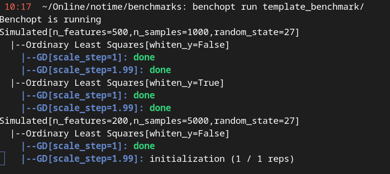
../_images/console_template.png — A screenshot of the console during the benchopt run command#

You will see something similar to the screenshot above in your terminal

Simulated tells us that the dataset run by benchopt is the simulation set up in the benchmark.

Ordinary Least Squares tells us which loss is minimized, and the hyperparameters are written in bracket.

GD is a line indicating the progress of algorithm GD for this problem (Simulated dataset, OLS loss). Again its hyperparameters are written in brackets (here the stepsize value).

Once the benchmark has been run, a window should open in your default navigator. This provides a visualization of the results of the run, which is useful to immediately observe, comment and share the results. After running the template benchmark, we can observe the convergence plots of GD with the two different stepsize choices, for two different simulated datasets.

The convergence plot scales can be changed for easier reading. In this specific toy example, the runtime is so low that the convergence plot with respect to time may not be reliable: you can also look at the results in terms of iterations, by scrolling the menu on the bottom left of the webpage. Feel free to play around with the plotting options here! Note that the objective comes with two possible values for a whiten parameter. Let us ignore this detail in the tutorial.

Exploring the benchmark structure#

The template benchmark we are using at the moment is not exactly encoding the information we need for the ridge regression problem. To properly modify the benchmark, first we need to dive deeper into how benchmarks work. To follow through this section, it is advised to open an editor (like vscode) at the root of the template benchmark to easily navigate between the files and folders.

Here is the architecture of our template benchmark (files which are not mandatory were ignored):

template_benchmark
├── datasets
│   └── simulated.py
├── solvers
│   └── python-gd.py
├── benchmark_utils
│   └── __init__.py
├── outputs
│   └── ...
├── objective.py
├── README.rst

The three most important files are

objective.py: it contains the information about the cost function we want to minimize. In other words, it defines the formal problem we are interested in.

solvers/python-gd.py: it contains the information and code for the gradient descent solver, dedicated to the problem at hand.

datasets/simulated.py: it contains the information about the dataset, i.e. the values of \(y \) and \(X \) used to test the algorithms. All benchmark in fact must have a simulated.py file which is used for testing by Benchopt.

Any benchmark must implement these three components; in Benchopt indeed we consider that objectives, solvers and dataset are the building blocks of any optimization problem.

There can be several solvers in the solvers/ directory, and similarly there can be several datasets in the datasets/ directory. Benchopt will then run all the solvers for each dataset. The other files are not very important right now, let us forget about them.

The content of objective.py, solvers and dataset is predetermined. In particular these three files each define a class inherited from Benchopt. The following figure details the methods that must be implemented in each file, and the order in which Benchopt will call these methods:

https://raw.githubusercontent.com/benchopt/communication_materials/main/sharedimages/benchopt_schema_dependency.svg

There are two kind of contents. First, code that defines core elements of the problem:

the evaluate_result method in objective.py. It implements the loss function. For the template benchmark, this is exactly \(g(\beta) \) when \( \beta \) is provided as input:
def evaluate_result(self, beta):
    diff = self.y - self.X @ beta
    return dict(
        value=.5 * diff.dot(diff)
    )
the run method in each solver, here python-gd. It defines the steps taken by the algorithm. Benchopt dictates the maximal number of iterations to the solver, and therefore run takes the number of iterations as input while other parameters like the stepsize are class attributes. The estimate value of \(\beta \) is updated in the class attributes, the run method does not require returns. For GD, the run function looks like
def run(self, n_iter):
    L = np.linalg.norm(self.X, ord=2) ** 2
    alpha = self.scale_step / L
    beta = np.zeros(self.X.shape[1])
    for _ in range(n_iter):
        beta -= alpha * gradient_ols(self.X, self.y, beta)

    self.beta = beta
the get_data method in simulated.py where \(y \) and \(X \) are defined. In this template benchmark, they are simply generated randomly using numpy.
def get_data(self):
    rng = np.random.RandomState(self.random_state)
    X = rng.randn(self.n_samples, self.n_features)
    y = rng.randn(self.n_samples)
    return dict(X=X, y=y)

The second type of methods found in these three python files are the communication tools. Indeed, solvers, dataset and objectives need to exchange information. Typically, the solver needs to know the parameters used for the loss, in our case the value of the regularization parameter. The objective needs to know the values of \( X\) and \( y\) defined in the dataset. This part of the benchmark can be hard to comprehend if you are not familiar with the structure of the benchmark, but the figure above should be a good reference point. When a method from a class feeds a method in another class, it returns a dictionary (such as get_data we just discussed), otherwise it simply updates the class attributes.

Finally, one may wonder where to define the hyperparameters of the problem. The general rule of thumb is that hyperparameters are defined as attributes of solvers, objectives or dataset depending on where it makes the most sense. For instance the stepsize is a solver-dependent parameter, it is defined as an attribute of the python-gd solver

class Solver(BaseSolver):
    name="GD"
    parameters = {
        'scale_step': [1, 1.99]
    }

Updating the template to implement a ridge regression benchmark#

We are now equipped with enough knowledge to update the template benchmark to a ridge regression benchmark. Formally, we are starting from OLS and GD implemented for the OLS problem. Therefore we need to implement the following modifications:

we should add the regularization term \( +\lambda \|\beta \|^2 \) to the loss in objective.py, and values for the regularization parameter.

we should modify the computed gradient, knowing that \( \nabla f(\beta) = \nabla g(\beta) + 2\lambda\beta \).

We will not modify anything in the dataset since the inputs \(X,y \) of the regression and ridge regression are the same.

Let’s start with the objective.py file. The regularization parameter values are part of the formal definition of the problem, so we can define them as attributes of the Objective class. In other words, we can simply add a reg parameter in the parameters dictionary to tell benchopt to grid over this parameter in the runs. The whiten_y parameter is not useful for us here, and we will remove the True option.

class Objective(BaseObjective):
    name = "Ordinary Least Squares"
    parameters = {
        'whiten_y': [False],
        'reg': [1e1, 1e2]
    }

This piece of code says that \( \lambda\) should take two values, \( 10\) or \( 100\), in the benchmark.

Then we update the evaluate_result method as follows:

def evaluate_result(self, beta):
    diff = self.y - self.X.dot(beta)
    l2reg = self.reg*np.linalg.norm(beta)**2
    return dict(
        value=.5 * diff.dot(diff) + l2reg,
        ols=.5 * diff.dot(diff),
        penalty=l2reg,
    )

We have done several modifications here:

The l2reg variable computes the regularization term. It is added to the OLS term in the value field of the output dictionary. This value field is the main loss of the benchmark, used by all algorithms to track convergence. In fact the naming convention here matters, by default the main loss must be named value.

Additional metrics are computed, namely ols and penalty. Benchmark will compute these metrics alongside the loss function, and we will be able to look at them in the resulting plots.

One additional modification handles the fact that the solvers will require the knowledge of \(\lambda\). The way to communicate from objectives to solvers, according to the figure above, is by using the get_objective method. It can be modified as follows

def get_objective(self):
    return dict(
        X=self.X,
        y=self.y,
        reg=self.reg
    )

Moreover we should also change the name of the objective from Ordinary Least Squares to Ridge Regression in the attributes of the Objective class in objective.py.

class Objective(BaseObjective):
    name = 'Ridge Regression'

That’s it for the objective.py file! We can now modify the solver. For simplicity we may directly edit python-gd.py, but adding a new solver to the benchmark is a simple as adding another file in the solvers folder (more information in the add a solver tutorial).

Modifying the solver means updating the run method, more specifically the gradient formula. Inside the python-gd.py file, the new run method looks like this

def run(self, n_iter):
    L = np.linalg.norm(self.X, ord=2) ** 2 + 2*self.reg
    alpha = self.scale_step / L
    beta = np.zeros(self.X.shape[1])
    for _ in range(n_iter):
        beta -= alpha * (gradient_ols(self.X, self.y, beta) + 2*self.reg*beta)

    self.beta = beta

Note that we are using self.reg as the value of \( \lambda \). To get this value from the objective.py file, we need to update the set_objective method, which is the counterpart of get_objective we just updated in objective.py.

def set_objective(self, X, y, reg):
    self.X, self.y, self.reg = X, y, reg

As a final step, because the goal of this benchmark is to look at GD performance for various hyperparameters, and in particular the stepsize, we are interested in setting the stepsize grid. The values taken by the stepsize are defined as attributes of the solver GD class, since they are parameters of the solver. Let us add scaled values 0.1 and 0.5 to the stepsize grid.

class Solver(BaseSolver):
    name = 'GD'
    parameters = {
        'scale_step': [0.1, 0.5, 1, 1.99],
    }

And that’s it, you now have your first benchmark setup! Congratulations :)

All that’s left is to run the benchmark and look at the results. We run the benchopt with the same command as earlier, in the parent directory of the template benchmark:

benchopt run my_benchmark

Notice how the prompt in the terminal now contains logging for the GD algorithm with each stepsize 0.1, 0.5, 1 and 1.99.

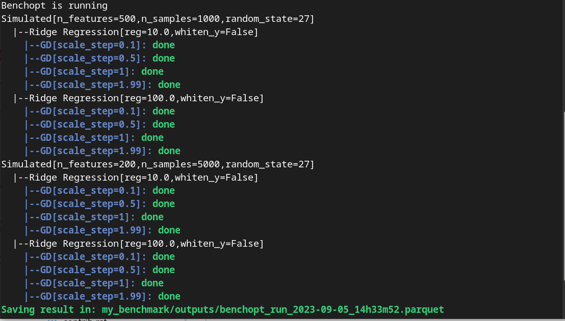
../_images/console_ridge.png — Screenshot of the console after running the updated benchmark.#

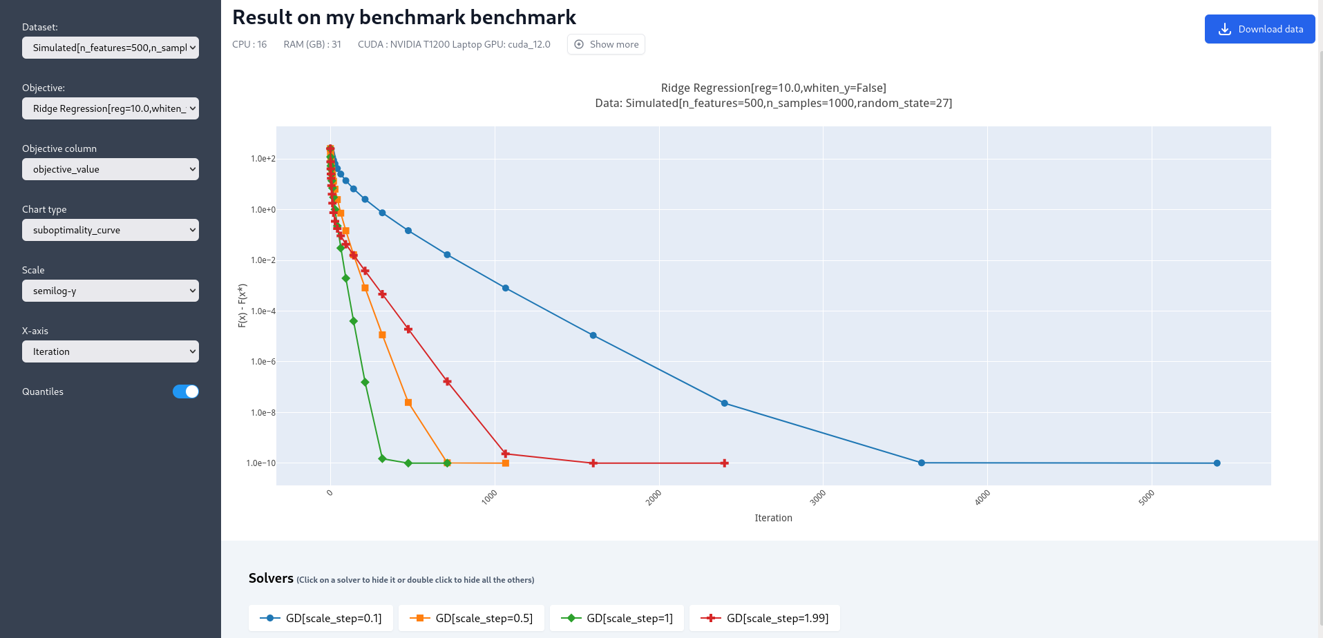
Upon completion of the run, you should again have all the results collected in a new interactive window in your default web navigator. There is a lot of interesting information contained in these results. For instance, select the following plotting options:

Simulated[n_features=500, n_samples=1000]

Ridge Regression[reg=10.0, whiten_y=False]

objective_value

suboptimality_curve

semilog-y

iteration

You should see the following plot (click image to zoom).

We may observe that the GD-ridge with stepsize=1 reaches a low cost value faster that when using smaller or larger stepsize. This is expected since the stepsize has been scaled optimally according to the theory of convex optimization, and therefore stepsize=1 is in principle the fastest safe step.

One of the interesting features of Benchopt is its ability to easily compute and show several metrics over the run. We have computed the ridge penalization alongside the iterations, and we can observe its values by changing the Objective_column field to objective_penalty. For better visualisation, you may change the Scale field to semilog-x. Observe that the ridge regularisation term increases with the iterations. Again this is expected since we initialized GD with a null vector for which the Euclidean norm is zero.

Concluding remarks#

Thank you for completing this tutorial! Hopefully your understanding of Benchopt benchmark is now sufficient to start your own benchmark. You may find more information in the online documentation about writing a benchmark. Moreover, there are a lot of other interesting features to Benchopt, feel free to go over the online documentation to learn more about Command Line Interface, publishing benchmark results, or configuring Benchopt.

As a final word, for simplicity, the way we cloned the template_benchmark repository to create our benchmark slightly differs from the recommended procedure. Instead, to start you benchmark, follow the instructions found in the README.rst file.

Understanding and building a simple benchmark

Contents