Visualize a benchmark

After running a benchmark, benchopt automatically displays the results in an HTML dashboard. Let’s explore the dashboard features on the Lasso benchmark.

Hint

Head to Get started to first install benchopt and setup the Lasso benchmark.

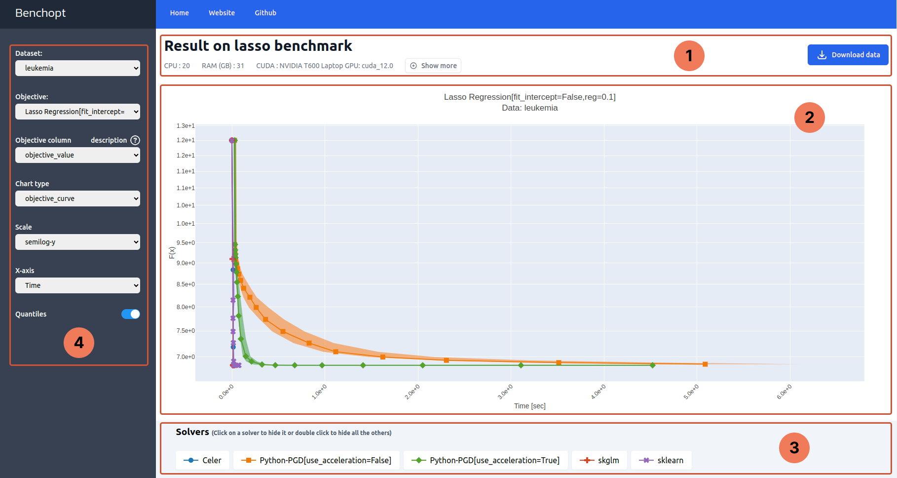
Part 1: Header

Part 1 contains the benchmark metadata: the benchmark title and the specifications of the machine used to run it. On the right hand side is a Download button to download the results of the benchmark as .parquet file.

Part 2: Figure

Part 2 is the main figure that plots the tracked metrics throughout the benchmark run. Its title shows the objective and the dataset names and their corresponding parameters that produced the plot.

Hovering over the figure will make a modebar appear in the right side. This can be used to interact with the figure, e.g. zoom in and out on particular regions of the plot.

Part 3: Legend

The legend maps every curve to a solver.

Clicking on a legend item hides/shows its corresponding curve. Similarly, double-clicking on a legend item hides/shows all other curves. Finally, hovering over a legend item shows a tooltip with details about the solver.

Note

The displayed details about the solver are the content of the solver’s docstring, if present.

Part 4: Sidebar

The first two dropdown menus, Data and Objective, enable to select a benchmark setup. The Data dropdown contains all the datasets included in the benchmark as well as their parameters. The same as for Objective dropdown.

The Objective column exposes all the tracked metrics along the benchmark run. These metrics are the ones defined in the Objective and correspond to the quantities returned by Objective.evaluate_result.

Hovering over the question mark shows a tooltip with details about the objective. Like solver, the details are the content of the Objective docstring.

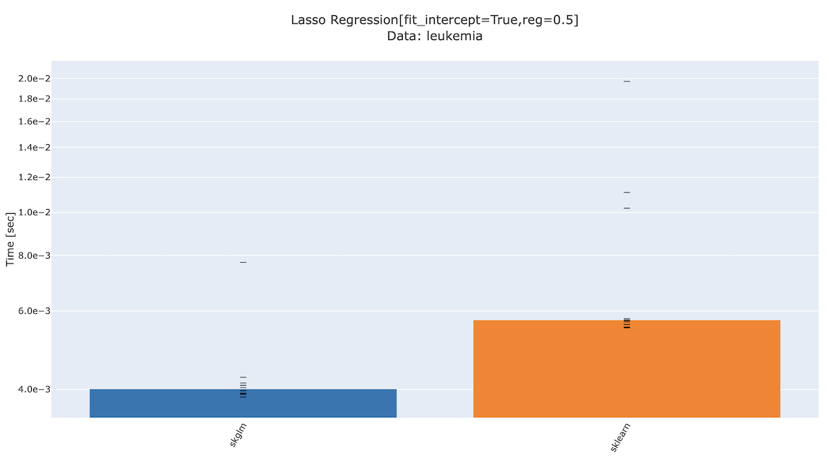
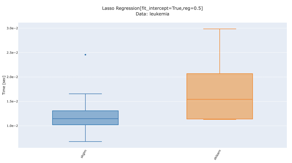
The Chart type dropdown allows applying transformations to the plotted metric, such as suboptimality metric - min(metric) or relative suboptimality (metric - min(metric)) / (metric[0] - min(metric)).

Note

For suboptimality plots, min(metric) is evaluated across all solvers and iterations. If no solver converged, it does not represent the minimal value reachable.

Use Scale to set x and y axis scale to linear or logarithmic.

Similarly, use X-axis to change the quantity plotted in the x-axis and therefore plotting the metric as a function of time, iteration or tolerance.

Note

The availability of Iteration, and Tolerance in the dropdown menu depends on the sampling strategy used for the solvers. Also, their interpretation is solver-dependent.

Finally, Quantiles is a toggler to show/hide 95th - 5th quantiles when the benchmark was run with several repetitions.