Configure views in a benchmark’s visuzalization

This example shows how to configure views in a benchmark visualization with config.yml and how to add custom plots to your benchmark.

# Import example helpers to define benchmarks and run benchopt in this example
from benchopt.helpers.run_examples import ExampleBenchmark
from benchopt.helpers.run_examples import benchopt_cli

Start with a minimal benchmark, including an objective, one dataset and one solver. This benchmark has no config.yml file specifying plotting options.

benchmark = ExampleBenchmark(
    base="minimal_benchmark", name="minimal_benchmark",
    ignore=["custom_plot.py", "example_config.yml", "config.yml"]
)
benchmark

            


                

                    ⬇ Download

                    objective.py
from benchopt import BaseObjective
import numpy as np


class Objective(BaseObjective):
    # Name of the Objective function
    name = 'Quadratic'

    # The three methods below define the links between the Dataset,
    # the Objective and the Solver.
    def set_data(self, X):
        """Set the data from a Dataset to compute the objective.

        The argument are the keys of the dictionary returned by
        ``Dataset.get_data``.
        """
        self.X = X

    def get_objective(self):
        "Returns a dict passed to ``Solver.set_objective`` method."
        return dict(X=self.X)

    def evaluate_result(self, X_hat):
        """Compute the objective value(s) given the output of a solver.

        The arguments are the keys in the dictionary returned
        by ``Solver.get_result``.
        """
        return dict(value=np.linalg.norm(self.X - X_hat))

    def get_one_result(self):
        """Return one solution for which the objective can be evaluated.

        This function is mostly used for testing and debugging purposes.
        """
        return dict(X_hat=1)


datasets/simulated.py
from benchopt import BaseDataset

import numpy as np


class Dataset(BaseDataset):
    # Name of the Dataset, used to select it in the CLI
    name = 'simulated'

    # ``get_data()`` is the only method a dataset should implement.
    def get_data(self):
        """Load the data for this Dataset.

        Usually, the data are either loaded from disk as arrays or Tensors,
        or a dataset/dataloader object is used to allow the models to load
        the data in more flexible forms (e.g. with mini-batches).

        The dictionary's keys are the kwargs passed to ``Objective.set_data``.
        """
        return dict(X=np.random.randn(10, 2))


solvers/gd.py
from benchopt import BaseSolver
import numpy as np


class Solver(BaseSolver):
    # Name of the Solver, used to select it in the CLI
    name = 'gd'

    # By default, benchopt will evaluate the result of a method after various
    # number of iterations. Setting the sampling_strategy controls how this is
    # done. Here, we use a callback function that is called at each iteration.
    sampling_strategy = 'callback'

    # Parameters of the method, that will be tested by the benchmark.
    # Each parameter ``param_name`` will be accessible as ``self.param_name``.
    parameters = {'lr': [1e-3, 1e-2]}

    # The three methods below define the necessary methods for the Solver, to
    # get the info from the Objective, to run the method and to return a
    # result that can be evaluated by the Objective.
    def set_objective(self, X):
        """Set the info from a Objective, to run the method.

        This method is also typically used to adapt the solver's parameters to
        the data (e.g. scaling) or to initialize the algorithm.

        The kwargs are the keys of the dictionary returned by
        ``Objective.get_objective``.
        """
        self.X = X
        self.X_hat = np.zeros_like(X)

    def run(self, cb):
        """Run the actual method to benchmark.

        Here, as we use a "callback", we need to call it at each iteration to
        evaluate the result as the procedure progresses.

        The callback implements a stopping mechanism, based on the number of
        iterations, the time and the evoluation of the performances.
        """
        while cb():
            self.X_hat = self.X_hat - self.lr * (self.X_hat - self.X)

    def get_result(self):
        """Format the output of the method to be evaluated in the Objective.

        Returns a dict which is passed to ``Objective.evaluate_result`` method.
        """
        return {'X_hat': self.X_hat}


                
            
"
        

Run the benchmark to generate results. This will display a first HTML page based on benchopt’s default plotting configuration.

benchopt_cli(
    f"run {benchmark.benchmark_dir} -n 40 -r 2 -s gd[lr=[1e-1,3e-2,1e-2,3e-3]]"
)

$ benchopt run temp_benchmark_3i6ha6l1/minimal_benchmark -n 40 -r 2 -s gd[lr=[1e-1,3e-2,1e-2,3e-3]]

Benchopt is running!
Benchopt called using profiling
Loading objective, datasets and solvers... done.
simulated
  |--Quadratic
No seed was specified. Selected global seed: 0
    |--gd[lr=0.1]: done
    |--gd[lr=0.03]: done
    |--gd[lr=0.01]: done
    |--gd[lr=0.003]: done
Saving result in: 
temp_benchmark_3i6ha6l1/minimal_benchmark/outputs/benchopt_run_2026-05-28_01h0
2m14.parquet
Rendering benchmark results...
   Processing
temp_benchmark_3i6ha6l1/minimal_benchmark/outputs/benchopt_run_2026-05-28_01h0
2m14.parquet
done
Writing results to
temp_benchmark_3i6ha6l1/minimal_benchmark/outputs/minimal_benchmark_benchopt_r
un_2026-05-28_01h02m14.html
Writing minimal_benchmark index to
temp_benchmark_3i6ha6l1/minimal_benchmark/outputs/minimal_benchmark.html

The default plots are generated from the results, showing the evolution of the first key of the objective against time. Options in the Change plot> menu or the side bar allow to change this plot, changing the objective key, the x-axis or scale, or the type of plot. However, these options are reset when reloading the page. The concept of views allows to save specific configurations of the plot, that can be easily loaded.

In practice, you can create these interactively from the HTML result using the Save as view button once you have a view that is representative of your benchmark, then hit the Configs button in the Download area and save the file as a new config.yml in your benchmark. You can also directly write the config.yml file, as shown below.

Here, we define two simple views in config.yml. The first one is a log-log evolution plot, showing the objective curve as a function of time, while the second one is a bar chart showing the runtime of each solver. When defining a view, part of the plotting parameters can be left free. They will be kept as they are when activating the view.

benchmark.update(extra_files={
    "config.yml": '''
    plot_configs:
      Subopt. (log):
        plot_kind: objective_curve
        scale: loglog
      Runtimes:
        plot_kind: bar_chart
    '''
})

            

                
We now update the following files:


                

                    ⬇ Download

                    config.yml
plot_configs:
  Subopt. (log):
    plot_kind: objective_curve
    scale: loglog
  Runtimes:
    plot_kind: bar_chart


                
            
"
        

To re-generate the HTML report from the latest results, call benchopt plot. This will override the existing HTML page, which now has two views available in Available plot view at the top of the page, and the first view automatically loaded.

benchopt_cli(f"plot {benchmark.benchmark_dir}")

$ benchopt plot temp_benchmark_3i6ha6l1/minimal_benchmark

Rendering benchmark results...
   Processing
temp_benchmark_3i6ha6l1/minimal_benchmark/outputs/benchopt_run_2026-05-28_01h0
2m14.parquet
done
Writing results to
temp_benchmark_3i6ha6l1/minimal_benchmark/outputs/minimal_benchmark_benchopt_r
un_2026-05-28_01h02m14.html
Writing minimal_benchmark index to
temp_benchmark_3i6ha6l1/minimal_benchmark/outputs/minimal_benchmark.html

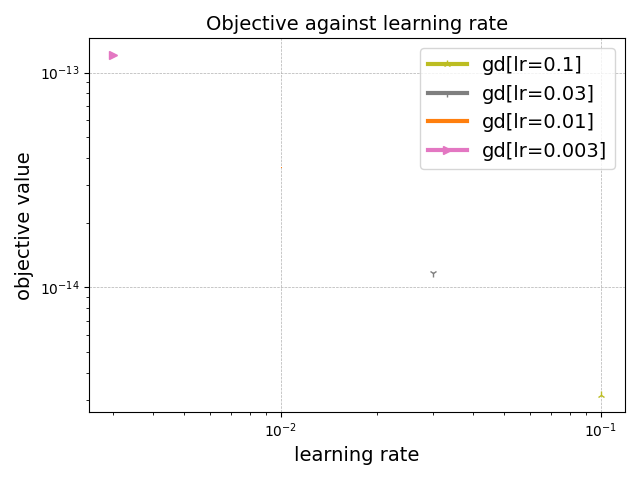
In some cases, the default plots are not suitable to visualize the results. With benchopt. It is possible to define custom plots that integrate seamlessly with the HTML interface. Here, we define a custom plot that shows the final objective value achieved by each solver against the runtime, with colors defined by the value of the learning rate used by the solver.

benchmark.update(plots={
    "custom_objective_time.py": '''
    from benchopt import BasePlot


    class Plot(BasePlot):
        name = "custom_objective_time"
        type = "scatter"
        options = {}

        def plot(self, df):
            points = []
            for solver in df['solver_name'].unique():
                sub_df = df.query("solver_name == @solver").sort_values('time')
                points.append({
                    "x": sub_df["p_solver_lr"].iloc[-1:].tolist(),
                    "y": sub_df["objective_value"].iloc[-1:].tolist(),
                    "label": solver,
                    **self.get_style(solver),
                })
            return points

        def get_metadata(self, df):
            return {
                "title": "Objective against learning rate",
                "xlabel": "learning rate",
                "ylabel": "objective value",
            }
    '''
})

            

                
We now update the following files:


                

                    ⬇ Download

                    plots/custom_objective_time.py
from benchopt import BasePlot


class Plot(BasePlot):
    name = "custom_objective_time"
    type = "scatter"
    options = {}

    def plot(self, df):
        points = []
        for solver in df['solver_name'].unique():
            sub_df = df.query("solver_name == @solver").sort_values('time')
            points.append({
                "x": sub_df["p_solver_lr"].iloc[-1:].tolist(),
                "y": sub_df["objective_value"].iloc[-1:].tolist(),
                "label": solver,
                **self.get_style(solver),
            })
        return points

    def get_metadata(self, df):
        return {
            "title": "Objective against learning rate",
            "xlabel": "learning rate",
            "ylabel": "objective value",
        }


                
            
"
        

This custom plot is rendered using a scatter plot, as disclosed in type. The get_metadata method defines global options for the plot, like the title and the axis labels, while the plot method defines the data to be plotted. For a scatter plot, this corresponds to a list of points or curves, with their x and y coordinates, labels and colors. The options attribute is empty here, but it can be used to define user-configurable options for the plot, that will be displayed in the HTML. More details on the plot API can be found in Add a custom plot to a benchmark.

We can then update plot_configs to include one view for the new custom plot, and run benchopt plot again to update the plot.

benchmark.update(extra_files={
    "config.yml": '''
    plot_configs:
      Sensitivity lr:
        plot_kind: custom_objective_time
        scale: loglog
      Subopt. (log):
        plot_kind: objective_curve
        scale: loglog
      Runtimes:
        plot_kind: bar_chart
    '''
})

            

                
We now update the following files:


                

                    ⬇ Download

                    config.yml
plot_configs:
  Sensitivity lr:
    plot_kind: custom_objective_time
    scale: loglog
  Subopt. (log):
    plot_kind: objective_curve
    scale: loglog
  Runtimes:
    plot_kind: bar_chart


                
            
"
        

Now running benchopt plot again will update the HTML page with the new plot option and the new view, showing the sensitivity of the final objective value to the selection of the learning rate.

benchopt_cli(f"plot {benchmark.benchmark_dir}")

$ benchopt plot temp_benchmark_3i6ha6l1/minimal_benchmark

Rendering benchmark results...
   Processing
temp_benchmark_3i6ha6l1/minimal_benchmark/outputs/benchopt_run_2026-05-28_01h0
2m14.parquet
done
Writing results to
temp_benchmark_3i6ha6l1/minimal_benchmark/outputs/minimal_benchmark_benchopt_r
un_2026-05-28_01h02m14.html
Writing minimal_benchmark index to
temp_benchmark_3i6ha6l1/minimal_benchmark/outputs/minimal_benchmark.html

Note that you can also generate custom plot as pdf using the --no-html option:

benchopt_cli(
    f"plot {benchmark.benchmark_dir} -k custom_objective_time --no-html"
)

$ benchopt plot temp_benchmark_3i6ha6l1/minimal_benchmark -k custom_objective_time --no-html

Save custom_objective_time as:
temp_benchmark_3i6ha6l1/minimal_benchmark/outputs/custom_objective_time.pdf