Running an existing benchmark

This example demonstrates how to run an existing benchmark with benchopt.

# Import example helpers to define the benchmark and
# programmatically call the CLI.
from benchopt.helpers.run_examples import ExampleBenchmark
from benchopt.helpers.run_examples import benchopt_cli

We will use the minimal benchmark defined in the examples folder. The benchmark objective is a simple minimization task:

\[\min_{\hat{X}} \; \mathrm{MSE}(X, \hat{X})\]

We define:

• an Objective that evaluates MSE between X and X_hat;

• a Dataset that generates a random matrix X;

• a Solver that minimizes this objective with gradient descent. It is parametrized with parameter lr for the step size.

benchmark = ExampleBenchmark(
    base="minimal_benchmark", name="minimal_benchmark",
    ignore=["custom_plot.py", "example_config.yml"]
)
benchmark

            


                

                    ⬇ Download

                    objective.py
from benchopt import BaseObjective
import numpy as np


class Objective(BaseObjective):
    # Name of the Objective function
    name = 'Quadratic'

    # The three methods below define the links between the Dataset,
    # the Objective and the Solver.
    def set_data(self, X):
        """Set the data from a Dataset to compute the objective.

        The argument are the keys of the dictionary returned by
        ``Dataset.get_data``.
        """
        self.X = X

    def get_objective(self):
        "Returns a dict passed to ``Solver.set_objective`` method."
        return dict(X=self.X)

    def evaluate_result(self, X_hat):
        """Compute the objective value(s) given the output of a solver.

        The arguments are the keys in the dictionary returned
        by ``Solver.get_result``.
        """
        return dict(value=np.linalg.norm(self.X - X_hat))

    def get_one_result(self):
        """Return one solution for which the objective can be evaluated.

        This function is mostly used for testing and debugging purposes.
        """
        return dict(X_hat=1)


datasets/simulated.py
from benchopt import BaseDataset

import numpy as np


class Dataset(BaseDataset):
    # Name of the Dataset, used to select it in the CLI
    name = 'simulated'

    # ``get_data()`` is the only method a dataset should implement.
    def get_data(self):
        """Load the data for this Dataset.

        Usually, the data are either loaded from disk as arrays or Tensors,
        or a dataset/dataloader object is used to allow the models to load
        the data in more flexible forms (e.g. with mini-batches).

        The dictionary's keys are the kwargs passed to ``Objective.set_data``.
        """
        return dict(X=np.random.randn(10, 2))


solvers/gd.py
from benchopt import BaseSolver
import numpy as np


class Solver(BaseSolver):
    # Name of the Solver, used to select it in the CLI
    name = 'gd'

    # By default, benchopt will evaluate the result of a method after various
    # number of iterations. Setting the sampling_strategy controls how this is
    # done. Here, we use a callback function that is called at each iteration.
    sampling_strategy = 'callback'

    # Parameters of the method, that will be tested by the benchmark.
    # Each parameter ``param_name`` will be accessible as ``self.param_name``.
    parameters = {'lr': [1e-3, 1e-2]}

    # The three methods below define the necessary methods for the Solver, to
    # get the info from the Objective, to run the method and to return a
    # result that can be evaluated by the Objective.
    def set_objective(self, X):
        """Set the info from a Objective, to run the method.

        This method is also typically used to adapt the solver's parameters to
        the data (e.g. scaling) or to initialize the algorithm.

        The kwargs are the keys of the dictionary returned by
        ``Objective.get_objective``.
        """
        self.X = X
        self.X_hat = np.zeros_like(X)

    def run(self, cb):
        """Run the actual method to benchmark.

        Here, as we use a "callback", we need to call it at each iteration to
        evaluate the result as the procedure progresses.

        The callback implements a stopping mechanism, based on the number of
        iterations, the time and the evoluation of the performances.
        """
        while cb():
            self.X_hat = self.X_hat - self.lr * (self.X_hat - self.X)

    def get_result(self):
        """Format the output of the method to be evaluated in the Objective.

        Returns a dict which is passed to ``Objective.evaluate_result`` method.
        """
        return {'X_hat': self.X_hat}


config.yml
#loaded from minimal_benchmark/config.yml
plot_configs:
  Subopt. (log):
    plot_kind: objective_curve
    scale: loglog
  Runtimes:
    plot_kind: bar_chart


                
            
"
        

To run the benchmark, just execute:

benchopt_cli(f"run {benchmark.benchmark_dir} -n 20 -r 2")

$ benchopt run temp_benchmark_l2u93w34/minimal_benchmark -n 20 -r 2

Benchopt is running!
Benchopt called using profiling
Loading objective, datasets and solvers... done.
simulated
  |--Quadratic
No seed was specified. Selected global seed: 0
    |--gd[lr=0.001]: done (not enough run)
    |--gd[lr=0.01]: done (not enough run)
Saving result in: 
temp_benchmark_l2u93w34/minimal_benchmark/outputs/benchopt_run_2026-05-28_00h5
6m28.parquet
Rendering benchmark results...
   Processing
temp_benchmark_l2u93w34/minimal_benchmark/outputs/benchopt_run_2026-05-28_00h5
6m28.parquet
done
Writing results to
temp_benchmark_l2u93w34/minimal_benchmark/outputs/minimal_benchmark_benchopt_r
un_2026-05-28_00h56m28.html
Writing minimal_benchmark index to
temp_benchmark_l2u93w34/minimal_benchmark/outputs/minimal_benchmark.html

This runs the benchmark named minimal_benchmark located in the examples folder.

The parameters n controls the number of point on the curves, while r controls the number of repetitions for each solver. The repetitions are used to compute the median and quartiles of the curves.

To get a more precise curve, you can increase n and r:

benchopt_cli(f"run {benchmark.benchmark_dir} -n 30 -r 5")

$ benchopt run temp_benchmark_l2u93w34/minimal_benchmark -n 30 -r 5

Benchopt is running!
Benchopt called using profiling
Loading objective, datasets and solvers... done.
simulated
  |--Quadratic
No seed was specified. Selected global seed: 0
    |--gd[lr=0.001]: done
    |--gd[lr=0.01]: done
Saving result in: 
temp_benchmark_l2u93w34/minimal_benchmark/outputs/benchopt_run_2026-05-28_00h5
6m33.parquet
Rendering benchmark results...
   Processing
temp_benchmark_l2u93w34/minimal_benchmark/outputs/benchopt_run_2026-05-28_00h5
6m33.parquet
done
Writing results to
temp_benchmark_l2u93w34/minimal_benchmark/outputs/minimal_benchmark_benchopt_r
un_2026-05-28_00h56m33.html
Writing minimal_benchmark index to
temp_benchmark_l2u93w34/minimal_benchmark/outputs/minimal_benchmark.html

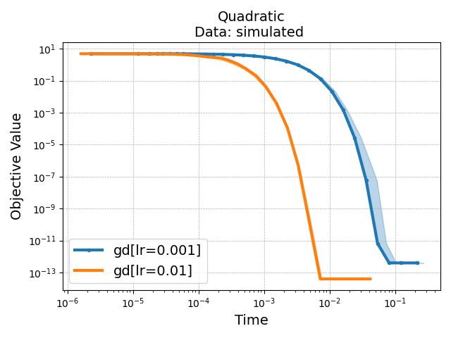
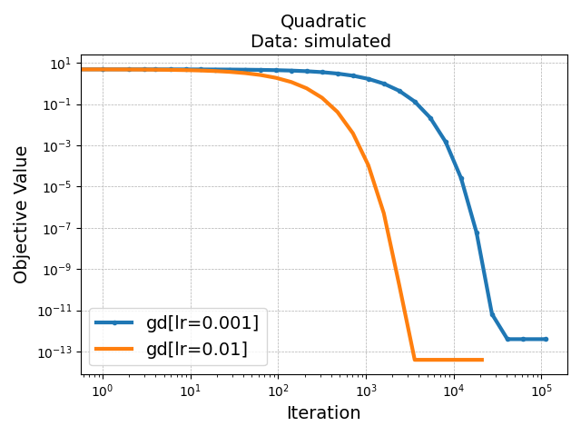
Here, the display is not ideal because both solvers reach convergence very quickly. You can change the display by selecting the scale of the axis in the plot configuration panel. Go to the Change plot banner at the top of the HTML file, and change the scale to loglog on the drop down menu.

Note that for convenience, this can be saved as a view in the configuration of the benchmark. See here for more details. Here, clicking on Subopt. (log) in the Available plots above the figure will take you to a view with the right scale, and looking at suboptimality instead of objective value.

Once the benchmark has be run, you can also generate pdf figures using the benchopt plot command with --no-html option:

benchopt_cli(
    f"plot {benchmark.benchmark_dir} -k objective_curve --no-html"
)

• 
• 

$ benchopt plot temp_benchmark_l2u93w34/minimal_benchmark -k objective_curve --no-html

Save objective_curve_simulated_Quadratic_objective_value_Time as:
temp_benchmark_l2u93w34/minimal_benchmark/outputs/objective_curve_simulated_Qu
adratic_objective_value_Time.pdf
Save objective_curve_simulated_Quadratic_objective_value_Iteration as:
temp_benchmark_l2u93w34/minimal_benchmark/outputs/objective_curve_simulated_Qu
adratic_objective_value_Iteration.pdf

See here for more details on how to customize the plots and define your own visualization.